Designing a Butterworth low-pass filter with SciPy

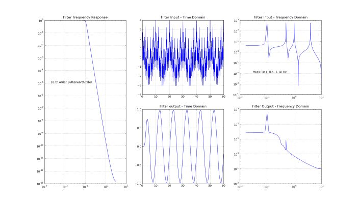
from scipy import signal
import math, numpy
from matplotlib import pyplot

# some constants
samp_rate = 20
sim_time = 60
nsamps = samp_rate*sim_time
cuttoff_freq = 0.1

fig = pyplot.figure()

# generate input signal
t = numpy.linspace(0, sim_time, nsamps)
freqs = [0.1, 0.5, 1, 4]
x = 0
for i in range(len(freqs)):
 x += numpy.cos(2*math.pi*freqs[i]*t)
time_dom = fig.add_subplot(232)
pyplot.plot(t, x)
pyplot.title('Filter Input - Time Domain')
pyplot.grid(True)

# input signal spectrum
xfreq = numpy.fft.fft(x)
fft_freqs = numpy.fft.fftfreq(nsamps, d=1./samp_rate)
fig.add_subplot(233)
pyplot.loglog(fft_freqs[0:nsamps/2], numpy.abs(xfreq)[0:nsamps/2])
pyplot.title('Filter Input - Frequency Domain')
pyplot.text(0.03, 0.01, "freqs: "+str(freqs)+" Hz")
pyplot.grid(True)

# design filter
norm_pass = cuttoff_freq/(samp_rate/2)
norm_stop = 1.5*norm_pass
(N, Wn) = signal.buttord(wp=norm_pass, ws=norm_stop, gpass=2, gstop=30, analog=0)
(b, a) = signal.butter(N, Wn, btype='low', analog=0, output='ba')
print("b="+str(b)+", a="+str(a))

# filter frequency response
(w, h) = signal.freqz(b, a)
fig.add_subplot(131)
pyplot.loglog(w, numpy.abs(h))
pyplot.title('Filter Frequency Response')
pyplot.text(2e-3, 1e-5, str(N)+"-th order Butterworth filter")
pyplot.grid(True)

# filtered output
#zi = signal.lfiltic(b, a, x[0:5], x[0:5])
#(y, zi) = signal.lfilter(b, a, x, zi=zi)
y = signal.lfilter(b, a, x)
fig.add_subplot(235)
pyplot.plot(t, y)
pyplot.title('Filter output - Time Domain')
pyplot.grid(True)

# output spectrum
yfreq = numpy.fft.fft(y)
fig.add_subplot(236)
pyplot.loglog(fft_freqs[0:nsamps/2], numpy.abs(yfreq)[0:nsamps/2])
pyplot.title('Filter Output - Frequency Domain')
pyplot.grid(True)

pyplot.show()